One Dimensional Low pass , High Pass and band pass filtering

Consider a one dimensional signal in time domain.

For instance, generate cosine waves of different amplitudes and different frequencies and combine them to form a complicated signal.

Consider four cosines waves with frequencies 23, 18, 10 and 5 and amplitudes 1.2, 0.8, 1.1 and 2 respectively and combine them to generate a signal.

Eg.

Cosine wave with frequency 23 and amplitude 1.2.

 

Figure.1

Cosine wave with frequency 18 and amplitude 0.8

 

Figure.2

Cosine wave with frequency 10 and amplitude 1.1

 

Figure.3

Cosine wave with frequency 5 and amplitude 2.

Figure.4

MATLAB code:

%To generate a signal

%Input function A cos(2pift)

freq =[23 18 10 5];

Amp = [1.2 0.8 1.1 2];

fs = 100;

ts = 1/fs;

t = 0:ts:5;

xt1 = 0;

for Ind = 1:numel(freq)

Freq = freq(Ind);

A = Amp(Ind);

xt1 = xt1+A*cos(2*pi*Freq*t);

end

figure,plot(t,xt1);

 

Figure.5

Let’s make a little understanding of this signal in frequency domain.

i.e in Fourier domain.

Fourier transform is one of the various mathematical transformations known which is used to transform signals from time domain to frequency domain.
The main advantage of this transformation is it makes life easier for many problems when we deal a signal in frequency domain rather than time domain.

After fourier transform, the signal will look like the below figure.

MATLAB code:

f1 = linspace(-fs/2,fs/2,numel(xt1));

xf = fftshift(fft(xt1));

str = 'Frequency domain';

figure,plot(f1,abs(xf)),title(str);

 

Figure.6

EXPLANATION:

In the figure.6, there are 4 different colors to denote four different signals.

Due to symmetric property, we see two peaks of the same signal.

fftshift is useful for visualizing the Fourier transform with the zero-frequency component in the middle of the spectrum.

The yellow color peaks denote the frequency with 5

The blue color peaks denote the frequency with 10

The green color peaks denote the frequency with 18

And the red color denotes the frequency with 23.

From this, we can understand that the low frequency components are close to the centre of the plot and the high frequency components are away from the centre.

Now, lets try to separate each of the original 4 signals from the combined ones.

We will keep only one signal at a time and remove/filter the rest.

MATLAB code:

       Kernel_BP = abs(f1) < 8;

   BPF = Kernel_BP .* xf;

  

   figure,plot(f1,abs(BPF));

Figure.7

Figure.8

A kernel is used to obtain the essential frequency component alone.

This can be done by making the values one for the frequency range less than 8 and rest zero.

We have obtained the lowest frequency component and the kernel we designed is for low pass filtering. The value which we use to find the limit is the cut off frequency. Here 8 is the cut of frequency.

Now , let’s go back to time domain.

MATLAB code:

BP_t = ifft(ifftshift(BPF));

plot(t,real(BP_t));

Compare the figure.4 and figure.9, both have same frequency right!!

Figure.9

Now let’s try to design the kernel for filtering high frequency component.

High Pass filter:MATLAB code :

    

   Kernel_BP = abs(f1) > 20;

   BPF = Kernel_BP .* xf;

  

   figure,plot(f1,abs(BPF));

 

Figure.10

   

Figure.11

  BP_t = ifft(ifftshift(BPF));

  plot(t,real(BP_t));

Figure.12

We have obtained the same signal as in figure.1

We will try to filter the signal of frequency 18.

This is band pass filter.

Band Pass Filter:
MATLAB code:

   Kernel_BP = abs(f1) > 15 & abs(f1) < 20;

   BPF = Kernel_BP .* xf;

  

   figure,plot(f1,abs(BPF));

         

Figure.13

   BP_t = ifft(ifftshift(BPF));

   plot(t,real(BP_t));

 

Figure.14

Figure.15

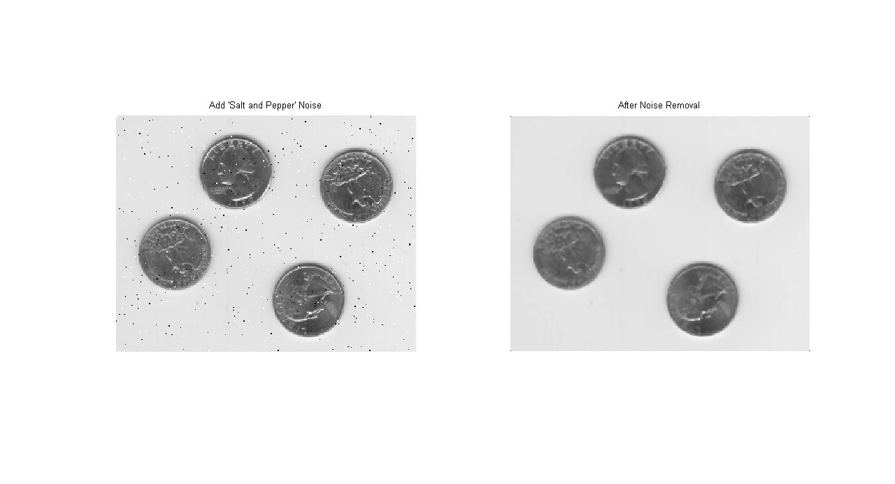
This same type of filtering can be applied on noisy signals to remove undesired signals.

MATLAB code:

Noise = 2 * randn(size(t));

xt1 = xt1 + Noise;

Using this signal as input, we can apply low, high and band pass to remove noise and obtain the original signal(to some extent).

Wait for my next post on two dimensional low and high pass filtering. i.e on images in space domain.

Gaussian Filter without using the MATLAB built_in function

Gaussian Filter

Gaussian Filter is used to blur the image. It is used to reduce the noise and the image details.

          The Gaussian kernel's center part  ( Here 0.4421 )  has the highest value and  intensity of other pixels  decrease as the distance from the center part increases.

               On convolution of the local region and the Gaussian kernel gives the highest intensity value to the center part of the local region(38.4624) and the remaining pixels have less intensity as the distance from the center increases.

               Sum up the result and store it in the current pixel location(Intensity = 94.9269) of the image.

MATLAB CODE:

%Gaussian filter using MATLAB built_in function

%Read an Image

Img = imread('coins.png');

A = imnoise(Img,'Gaussian',0.04,0.003);

%Image with noise

figure,imshow(A);

H = fspecial('Gaussian',[9 9],1.76);

GaussF = imfilter(A,H);

figure,imshow(GaussF);

MATLAB CODE for Gaussian blur WITHOUT built_in function:

%Read an Image

Img = imread('coins.png');

A = imnoise(Img,'Gaussian',0.04,0.003);

%Image with noise

figure,imshow(A);

 

Image with Noise

I = double(A);

%Design the Gaussian Kernel

%Standard Deviation

sigma = 1.76;

%Window size

sz = 4;

[x,y]=meshgrid(-sz:sz,-sz:sz);

M = size(x,1)-1;

N = size(y,1)-1;

Exp_comp = -(x.^2+y.^2)/(2*sigma*sigma);

Kernel= exp(Exp_comp)/(2*pi*sigma*sigma);

 

Gaussian Kernel 9x9 size with Standard Deviation =1.76

%Initialize

Output=zeros(size(I));

%Pad the vector with zeros

I = padarray(I,[sz sz]);

%Convolution

for i = 1:size(I,1)-M

    for j =1:size(I,2)-N

        Temp = I(i:i+M,j:j+M).*Kernel;

        Output(i,j)=sum(Temp(:));

    end

end

%Image without Noise after Gaussian blur

Output = uint8(Output);

figure,imshow(Output);

After Filtering

Min Filter - MATLAB CODE

MIN FILTER

•      To find the darkest points in an image.
•       Finds the minimum value in the area encompassed by the filter.
•       Reduces the salt noise as a result of the min operation.
•       The 0^th percentile filter is min filter.

The MIN Filtering is similar to MAX filter. Check MAX filter post to know how the formula is used to filter the pepper noise.

MATLAB CODE:

%READ AN IMAGE

A = imread('board.tif');

A = rgb2gray(A(1:300,1:300,:));

figure,imshow(A),title('ORIGINAL IMAGE');

%PREALLOCATE THE OUTPUT MATRIX

B=zeros(size(A));

%PAD THE MATRIX A WITH ZEROS

modifyA=padarray(A,[1 1]);

        x=[1:3]';

        y=[1:3]';

       

for i= 1:size(modifyA,1)-2

    for j=1:size(modifyA,2)-2

      

       %VECTORIZED METHOD 

       window=reshape(modifyA(i+x-1,j+y-1),[],1);

       %FIND THE MINIMUM VALUE IN THE SELECTED WINDOW

        B(i,j)=min(window);

    end

end

%CONVERT THE OUTPUT MATRIX TO 0-255 RANGE IMAGE TYPE

B=uint8(B);

figure,imshow(B),title('IMAGE AFTER MIN FILTERING');

Max Filter - MATLAB CODE

• To find the brightest points in an image.
•  Finds the maximum value in the area encompassed by the filter.
•  Reduces the pepper noise as a result of the max operation.
•  The 100^th percentile filter is max filter. Check the 50^th percentile filter i.e the median filter.

MATLAB CODE:

%READ AN IMAGE

A = imread('board.tif');

A = rgb2gray(A(1:300,1:300,:));

figure,imshow(A),title('ORIGINAL IMAGE');

%PREALLOCATE THE OUTPUT MATRIX

B=zeros(size(A));

%PAD THE MATRIX A WITH ZEROS

modifyA=padarray(A,[1 1]);

        x=[1:3]';

        y=[1:3]';

       

for i= 1:size(modifyA,1)-2

    for j=1:size(modifyA,2)-2

      

       %VECTORIZED METHOD

       window=reshape(modifyA(i+x-1,j+y-1),[],1);

       %FIND THE MAXIMUM VALUE IN THE SELECTED WINDOW

        

       B(i,j)=max(window);

   

    end

end

%CONVERT THE OUTPUT MATRIX TO 0-255 RANGE IMAGE TYPE

B=uint8(B);

figure,imshow(B),title('IMAGE AFTER MAX FILTERING');

Adaptive filtering-local noise filter

Adaptive filter is performed on the degraded image that contains original image and noise. The mean and variance are the two statistical measures that a local adaptive filter depends with a defined mxn window region. 

MATLAB CODE:

A = imread('saturn.png');

B = rgb2gray(A);

sz = size(B,1)*size(B,2);

%Add gaussian noise with mean 0 and variance 0.005

B = imnoise(B,'gaussian',0,0.005);

figure,imshow(B); title('Image with gaussian noise');

B = double(B);

%Define the window size mxn

M = 5;

N = 5;

%Pad the matrix with zeros on all sides

C = padarray(B,[floor(M/2),floor(N/2)]);

lvar = zeros([size(B,1) size(B,2)]);

lmean = zeros([size(B,1) size(B,2)]);

temp = zeros([size(B,1) size(B,2)]);

NewImg = zeros([size(B,1) size(B,2)]);

for i = 1:size(C,1)-(M-1)

    for j = 1:size(C,2)-(N-1)

        

        

        temp = C(i:i+(M-1),j:j+(N-1));

        tmp =  temp(:);

             %Find the local mean and local variance for the local region        

        lmean(i,j) = mean(tmp);

        lvar(i,j) = mean(tmp.^2)-mean(tmp).^2;

        

    end

end

%Noise variance and average of the local variance

nvar = sum(lvar(:))/sz;

%If noise_variance > local_variance then local_variance=noise_variance

 lvar = max(lvar,nvar);     

 %Final_Image = B- (noise variance/local variance)*(B-local_mean);

 NewImg = nvar./lvar;

 NewImg = NewImg.*(B-lmean);

 NewImg = B-NewImg;

 %Convert the image to uint8 format.

 NewImg = uint8(NewImg);

figure,imshow(NewImg);title('Restored Image using Adaptive Local filter');

Add salt and pepper noise to image

How to add salt and pepper noise to an image

          To obtain an image with ‘speckle’ or ‘salt and pepper’ noise we need to add white and black pixels randomly in the image matrix.

First convert the RGB image into grayscale image.

Then generate random values for the size of the matrix.

Here I used MATLAB function ‘randint’.

This function will generate random values for the given matrix size within the specified range.

For instance, consider an image matrix of size 4X3

Imgmatrix =

   237   107   166

   234    95   162

   239   116   169

   56   126    89

Generate random values for a 4X3 matrix with range 0 to 10.

randint(4,3,[0,10])

ans =

     4    10     4

     7     8     4

    10     0     5

     3    10     9

    

Now we can replace with pixel value zero (black) in the image matrix if there is ‘0’ value in the random matrix.

Now the image matrix will have black pixels.

Imgmatrix =

   237   107   166

   234    95   162

   239   0   169

   56   126    89

 

Similarly, replace the image matrix pixel value with ‘255’ if there is value ‘10’ in the random matrix.

The white pixels are now added.

Imgmatrix =

   237   255   166

   234    95   162

   255   0   169

   56   126    89

Black=0 white=255

 

MATLAB CODE:

A=imread('taj.jpg');

B=rgb2gray(A);

black=3;

white=253;

%Adjust the values in 'black' and 'white' to increase the noise.

NoiseImg = B;

    Rmatrix = randint(size(B,1),size(B,2),[0,255]);

    NoiseImg(Rmatrix <= black) = 0;

    NoiseImg(Rmatrix >=white) = 255;

    RImg=medfilt2(NoiseImg);

    figure,subplot(1,2,1),imshow(NoiseImg),title('Add ''Salt and Pepper'' Noise');

    subplot(1,2,2),imshow(RImg),title('After Noise Removal');

 I used the MATLAB function 'medfilt2' to remove noise. 

Learn how to remove the noise without using the 'medfilt2' function.