Upsampling in MATLAB

Upsampling is the process of inserting zeros in between the signal value in order to increase the size of the matrix.  We will discuss about upsampling in both spatial and time domain.

1.      Upsampling in Spatial Domain

1.1  Upsampling using MATLAB built-in function

1.2  Upsampling in 1D

1.3  Upsampling in 2D or image matrix

2.      Upsampling in Frequency Domain

2.1  Upsampling a 1D signal

2.2  Upsampling a image matrix

UPSAMPLING IN SPATIAL DOMAIN:

Given: 1-D array of size 1xN

Upsample by factor of 2:  

Output: 1-D array of size 1x(2*N)

Where N represents length of the array, n represents the index starting from 0,1,2…,N

%UPSAMPLING USING MATLAB BUILT-IN FUNCTION 'UPSAMPLE'

A = 1:25;

B = upsample(A,2);

EXPLANATION:

The above MATLAB function will insert zeros in between the samples.

To upsample an array by ratio 2, update the output array as follows:

1.      If index(n) of the output array is divisible by 2(ratio), then update the output array with the value of the input array with index n/2

2.      Otherwise, insert zero

STEPS TO PERFORM:

1.      Consider an array A of size 1xM

2.      Obtain the upsample Ratio N

3.      Pre-allocate an array B of size 1x(M*N)

4.      If the index is divisible by N then update the array B with value of A else zero

MATLAB CODE:

%UPSAMPLING IN SPATIAL DOMAIN

A = 1:10;

%UPSAMPLING WITH RATIO 2

B = zeros([1 size(A,2)*2]);

B(1:2:end)=A;

%UPSAMPLING WITH RATIO N

N=3;

B=zeros([1 size(A,2)*N]);

B(1:N:end)=A;

EXPLANATION:

Let A = [1 2 3 4 5]

Let us upsample try to upsample A with ratio 2

Pre-allocate output matrix B = [0 0 0 0 0 0 0 0 0 0]

Substitute the value of the matrix A in indices divisible by the ratio i.e. 2 of matrix B

B(1:2:end) = A

Now B(1,3,5,7,9) =[1 2 3 4 5]

Thus B = [1 0 2 0 3 0 4 0 5 0]

NOTE:

Definition of upsampling is usually given assuming the index starts from zero. But in case of MATLAB, the index starts with one that is why the odd positions are considered instead of even.

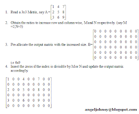
STEPS TO PERFORM TO UPSAMPLE A 2D MATRIX:

MATLAB CODE:

%IMAGE UPSAMPLING

A = imread('cameraman.tif');

M = 2;

N = 3;

B = zeros([size(A,1)*M size(A,2)*N]);

B(1:M:end,1:N:end) = A;

figure,imagesc(B);colormap(gray);

sz = M*N;

H = fspecial('average',[sz sz]);

C = conv2(B,H,'same');

figure,imagesc(C);colormap(gray);

EXPLANATION:

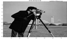
The above image is the pixel representation of the zero inserted image. In each row, two zeros are inserted between the pixels and in the each column; single zero is inserted between the pixels. In spatial domain, inserting zeros will be quite visible so it’s advisable to perform any low pass filtering or approximation like spatial averaging or applying Gaussian.

In the above example, spatial averaging is done. In order to understand how spatial averaging is done using convolution check the following link:

 http://angeljohnsy.blogspot.com/2015/11/convolution-in-matlab.html

UPSAMPLING IN FREQUENCY DOMAIN