Fast Fourier Transform on 2 Dimensional matrix using MATLAB

Fast Fourier transformation on a 2D matrix can be performed using the MATLAB built in function ‘fft2()’.

Fourier transform is one of the various mathematical transformations known which is used to transform signals from time domain to frequency domain.
The main advantage of this transformation is it makes life easier for many problems when we deal a signal in frequency domain rather than time domain.

Example:

%FOURIER TRANSFORM ON A MATRIX

A  = zeros(5);

A ( : ) = 1:25;

display(A);

F_FFT  = fft2(A);

display(F_FFT);

%INVERSE FOURIER TRANSFORM

I_FFT = ifft2(F_FFT);

display(abs(I_FFT));

NOTE on ABSOLUTE VALUE:

When we use FFT2() or FFT(),the result we obtain in the frequency domain is of complex data type.

i.e It contains both the real  as well as the imaginary part.

Let   A=10+5i

A is a complex number as it contains both real and imaginary part.In this particular case ‘10’ is the real part and ‘5’ is the imaginary part.

abs(A) = 11.1803 is the absolute (also called modulus in few books or notations) value of A which is nothing but the magnitude. It can be arrived by using the below mentioned formula:

abs(A) = sqrt(real part^2+imaginary part^2).

              = sqrt(10^2+5^2)

              = sqrt(125)

             = 11.1803 (approx)

Let’s try to understand how the Fourier transform on 2 dimensional data works with a simple example.

This method will be helpful to understand the up sampling and down sampling in both spatial and frequency domain.

1.       Consider a matrix A

2.       Perform 1 D Fast Fourier transform(FFT) on each row

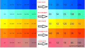
1D FFT on first row (Note that the absolute value is only displayed and not the actual imaginary number):

Similarly, perform  1D FFT on each row:

NOTE: The figure represents the 1 D FFT on each row and the result is the absolute value of the complex data obtained using FFT.

3.       Perform 1 D Fast Fourier transform on each column.
On the matrix obtained from the previous step, compute 1D FFT column wise.

4.       Display the results obtained.

Flow Chart for Fast Fourier Transform on 2D :

INVERSE FOURIER TRANSFORM:

1.       Perform Inverse Fourier Transform on each column

2.       Perform IFFT on each row

3.       Display the original data

MATLAB CODE:

A=[110 20 140 0 220;

   60 34 23 198 20;

   15 12 126 230 15;

   140 28 10 28 10;

   11 12 19 85 100];

FFT_row = zeros(size(A));

FFT_col = zeros(size(A));

%Perform FFT on each row

for i=1:size(A,1)

FFT_row(i,:) = fft(A(i,:));

end

display(FFT_row);

%display(abs(FFT_row));

%Perform FFT on each column

for i=1:size(A,2)

FFT_col(:,i) = fft(FFT_row(:,i));

end

display(FFT_col);

%display(abs(FFT_col));

%INVERSE FOURIER TRANSFORM

IFFT_row = zeros(size(A));

IFFT_col = zeros(size(A));

%Perform Inverse Fourier Transform on each column

for i=1:size(A,2)

IFFT_col(:,i) = ifft(FFT_col(:,i));

end

%Perform IFFT on each row

for i=1:size(A,2)

IFFT_row(:,i) = ifft(IFFT_col(:,i));

end

display(abs(A))

ALTERNATE METHOD FOR INVERSE FOURIER TRANSFORM:

Instead of using ifft2() or ifft(), we can also use the following method to obtain the original data from the Fast Fourier transformed result :

1.       Obtain the conjugate of the Forward FFT

2.       Perform Forward fast Fourier transform

3.       Obtain the conjugate of the result from step 2.

4.       Divide it by the number of elements present in the matrix

5.       Obtain the original matrix

MATLAB CODE:

Conj_F = conj(F_FFT);

Conj_FFT = fft2(Conj_F);

IFFT_conj = conj(Conj_FFT)/numel(Conj_FFT)

display(abs(IFFT_conj));

Reference: Digital Image Processing  by Rafael C.Gonzalez, fourth Chapter.